Consider a number, say 4. If we want to multiply this number by itself 3 times we can write this as either \(4 \times 4 \times 4\), or, more compactly, as \(4^3\). This operation is known as exponentiation and follows some well-known algebraic laws and conventions. For example, for any non-zero number \(x\) we have:
- \(x^k = \overbrace{x \times x \times \dots \times x}^{k \text{ times}}\)
- \(x^1 = x\)
- \(x^0 = 1\)
- \(x^{-1} = \frac{1}{x}\)
- \(x^{-k} = (\frac{1}{x})^{k}\)
This is all surely familiar to the reader. What may not be directly obvious, however, is that we can meaningfully define analogous operations on invertible matrices and use the same notation:
- \(A^k = \overbrace{AA \dots A}^{k \text{ times}}\): Exponentiation by positive integer is repeated multiplication.
- \(A^1 = A\): Exponentiation by identity returns original matrix.
- \(A^0 = I\): Exponentiation by zero returns the identity matrix.
- \(A^{-1} = \text{inv}(A)\): Exponentiation by -1 returns inverse of original matrix.
- \(A^{-k} = \text{inv}(A)^k\): Exponentiation by negative integer is repeated multiplication of inverse.
R does not have built-in support for these operations (e.g. for a matrix A, A^2 does not multiply A by itself, but rather squares every entry of A). In this post, therefore, we will implement this functionality. In doing so, we will touch on a number of topics:
- Defining test cases to make clear exactly what goal we’re trying to achieve, and test if our proposed solution achieves that goal
- Higher-order functions
- Using
purrr::reduceto avoid loops - Diagonalizing a matrix (which involves an eigendecomposition)
- Computational complexity
- Benchmarking code
Defining test cases
We start by loading some necessary packages.
library(tidyverse)
library(assertthat)
library(microbenchmark)
Next, we define a sample \(3 \times 3\) matrix that we use throughout the post.
set.seed(1)
n <- 3
(A <- matrix(sample(10, n ^ 2, TRUE), n, n))
## [,1] [,2] [,3]
## [1,] 3 10 10
## [2,] 4 3 7
## [3,] 6 9 7We now define a function test_properties that takes as input a matrix A and a function f that takes powers of that matrix. It then applies f to A for various exponents and checks if it gives the desired result. For example, for any implementation of a power function f we would expect that f(A, 0) (i.e. \(A\) raised to the zero power) would return the identity matrix (i.e. diag(1, nrow(A))).
test_properties <- function(f, A) {
  list(
    "A^4 == AAAA"      = are_equal(f(A,  4), A %*% A %*% A %*% A),
    "A^1 == A"         = are_equal(f(A,  1), A),
    "A^0 == I"         = are_equal(f(A,  0), diag(1, nrow(A))),
    "A^-1 == inv(A)"   = are_equal(f(A, -1), solve(A)),
    "A^-4 == inv(A)^4" = are_equal(f(A, -4), solve(A) %^% 4)
  )
}
Since test_properties is a function that takes another function as input, we would call this a higher-order function (or a functional to be more precise).
Strategy 1: Naive repeated multiplication
We can try out test_properties on a trivial implementation of a power function. (If the reader is unfamiliar with the percentage sign-notation, that is how we define infix functions in R).
`%^%` <- function(A, k) {
  A
}
So %^% takes an A and a k as input, throws away the k and returns the A unchanged. Let’s see what tests it passes.
str(test_properties(`%^%`, A))## List of 5
## $ A^4 == AAAA : logi FALSE
## $ A^1 == A : logi TRUE
## $ A^0 == I : logi FALSE
## $ A^-1 == inv(A) : logi FALSE
## $ A^-4 == inv(A)^4: logi FALSEIn order to pass all the other tests we need an implementation that actually does something. The next implementation starts by defining the identity matrix I of the same dimensions as A and initializes the matrix Ak to be this matrix (this is a bit roundabout, but useful for didactic purposes). It then enters a while-loop that decrements k while multiplying Ak by A. Once k hits zero, it returns the final matrix.
`%^%` <- function(A, k) {
  I <- diag(1, nrow(A))
  Ak <- I
  while(k > 0) {
    Ak <- Ak %*% A
    k <- k - 1
  }
  Ak
}

A %*% A
## [,1] [,2] [,3]
## [1,] 109 150 170
## [2,] 66 112 110
## [3,] 96 150 172A %^% 2## [,1] [,2] [,3]
## [1,] 109 150 170
## [2,] 66 112 110
## [3,] 96 150 172Let’s see if this implementation is any better.
str(test_properties(`%^%`, A))## List of 5
## $ A^4 == AAAA : logi TRUE
## $ A^1 == A : logi TRUE
## $ A^0 == I : logi TRUE
## $ A^-1 == inv(A) : logi FALSE
## $ A^-4 == inv(A)^4: logi FALSEOk, so it works for positive, but not negative, exponents. Let’s fix that.
`%^%` <- function(A, k) {
  I <- diag(1, nrow(A))
  if(k < 0) {
    A <- solve(A)
    k <- k * -1
  }
  Ak <- I
  while(k > 0) {
    Ak <- Ak %*% A
    k <- k - 1
  }
  Ak
}
Here we just check if k is negative, and if it is, replace A with its inverse. Everything else remains unchanged.
str(test_properties(`%^%`, A))## List of 5
## $ A^4 == AAAA : logi TRUE
## $ A^1 == A : logi TRUE
## $ A^0 == I : logi TRUE
## $ A^-1 == inv(A) : logi TRUE
## $ A^-4 == inv(A)^4: logi TRUEIt now passes all tests. Beautiful. As good functional programmers, however, we feel a bit queasy about using loops, so let’s use purrr::reduce to get rid of it.
`%^%` <- function(A, k) {
  I <- diag(1, nrow(A))
  if(k < 0) {
    A <- solve(A)
    k <- k * -1
  }
  reduce(seq_len(k), ~. %*% A, .init = I)
}
The first part here is identical to the earlier function, but instead of the while loop we call reduce on a dummy vector of length k with the identity matrix as the starting value. The machinery of reduce then takes care of all the details of accumulating the matrix products.
str(test_properties(`%^%`, A))## List of 5
## $ A^4 == AAAA : logi TRUE
## $ A^1 == A : logi TRUE
## $ A^0 == I : logi TRUE
## $ A^-1 == inv(A) : logi TRUE
## $ A^-4 == inv(A)^4: logi TRUEIndeed, the implementation with reduce also passes our test cases.
If we stop to consider how this appropach scales with larger inputs of k, however, we notice that we always need to do exactly k matrix multiplications. So the growth rate is linear in k. Since matrix multiplication itself is very computationally demanding – between \(\mathcal{O}(n^3)\) and \(\mathcal{O}(n^{2.373})\) depending on the algorithm – this approach will only work for fairly small matrices and small values of k. Fortunately, there’s a very clever approach that involves diagonalizing A which runs in much better time.
Strategy 2: Diagonalization
It’s a remarkable fact that under the right circumstances, a matrix \(A\) can be decomposed as \(A = PDP^{-1}\), where the columns of \(P\) are the eigenvectors of \(A\) and \(D\) is a diagonal matrix with the eigenvalues of \(A\) along the main diagonal.
Consider our matrix A. Let’s find its eigenvectors and eigenvalues.
eigen(A)## eigen() decomposition
## $values
## [1] 19.317668+0.000000i -3.158834+0.253746i -3.158834-0.253746i
##
## $vectors
## [,1] [,2] [,3]
## [1,] -0.6483318+0i -0.8600864+0.0000000i -0.8600864+0.0000000i
## [2,] -0.4288083+0i 0.2414274-0.2544460i 0.2414274+0.2544460i
## [3,] -0.6291179+0i 0.2882856+0.2326217i 0.2882856-0.2326217iSo \(A\) has three eigenvalues (which happen to be complex numbers) and three associated eigenvectors. If what we said above about the eigendecomposition is true, we should thus be able to do the following:
eig <- eigen(A)
P <- eig$vectors
P_inv <- solve(P)
D <- diag(eig$values)

A
## [,1] [,2] [,3]
## [1,] 3 10 10
## [2,] 4 3 7
## [3,] 6 9 7P %*% D %*% P_inv## [,1] [,2] [,3]
## [1,] 3-0i 10+0i 10-0i
## [2,] 4-0i 3+0i 7-0i
## [3,] 6-0i 9+0i 7-0iRe(P %*% D %*% P_inv)## [,1] [,2] [,3]
## [1,] 3 10 10
## [2,] 4 3 7
## [3,] 6 9 7So we indeed have \(A = PDP^{-1}\) (since the eigenvalues are in \(\mathbb{C}\) we have to coerce them back to \(\mathbb{R}\) using the Re function).
Now, not all matrices can be decomposed like this and the exact conditions for when a matrix is diagonalizable is a bit involved (we would have to figure out both the algebraic and geometric multiplicity of each eigenvalue, and check if they are all equal). However, there is a sufficient (but not necessary) condition for diagonalizability, viz. that an \(n \times n\) matrix is always diagonalizable if it has \(n\) distinct eigenvalues. So checking for this condition should deal with most situations. (We will ignore issues of numeric stability).
But how does all this help us with the problem of taking powers of a matrix?
Observe:
\[ A^2 = AA = PDP^{-1}PDP^{-1} = PD(P^{-1}P)DP^{-1} = PDIDP^{-1} = PDDP^{-1} = PD^2P^{-1} \]
More generally, \(A^n = PD^nP^{-1}\). And since \(D\) is diagonal, we can get \(D^n\) by simply raising the elements on the diagonal of \(D\) to \(n\), which is a very cheap operation. No messy repeated matrix multiplication!

Let’s write an implementation.
`%^^%` <- function(A, k) {
  eig <- eigen(A)

  # check if A is diagonalizable
  stopifnot(length(unique(eig$values)) == nrow(A))

  P <- eig$vectors
  D <- diag(eig$values ^ k)
  Ak <- P %*% D %*% solve(P)
  Re(Ak)
}
Let’s see if works.
str(test_properties(`%^^%`, A))## List of 5
## $ A^4 == AAAA : logi TRUE
## $ A^1 == A : logi TRUE
## $ A^0 == I : logi TRUE
## $ A^-1 == inv(A) : logi TRUE
## $ A^-4 == inv(A)^4: logi TRUELet’s also check it for some other matrix. Let \(B\) be the rotate-by-90-degrees-counterclockwise matrix. We would then expect \(B^4\) to be a full 360 degree turn, which is equivalent to doing nothing (i.e. the identity matrix).
(B <- matrix(c(0, 1, -1, 0), 2))## [,1] [,2]
## [1,] 0 -1
## [2,] 1 0B %^^% 4## [,1] [,2]
## [1,] 1 0
## [2,] 0 1str(test_properties(`%^^%`, B))## List of 5
## $ A^4 == AAAA : logi TRUE
## $ A^1 == A : logi TRUE
## $ A^0 == I : logi TRUE
## $ A^-1 == inv(A) : logi TRUE
## $ A^-4 == inv(A)^4: logi TRUEComparing the two strategies
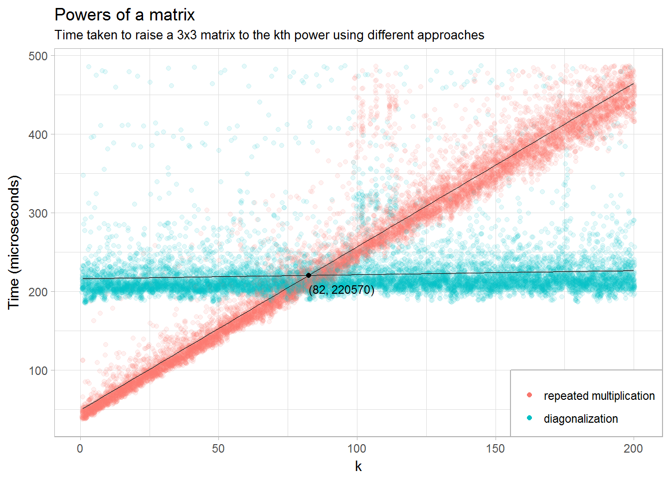
We would expect the run time of the first approach to be quite fast for small values of \(k\), since we don’t have to do any eigendecomposition, but to grow more or less linearly as \(k\) increases. Conversely, the second approach should be slow for small values of \(k\) since we have to find the eigenvalues and eigenvectors if even \(k\) is very small. But once that decomposition is found, the magnitude of \(k\) should have little effect on how long it takes to compute.
We set up a vector of k running from 1 to 200, and for each value we take A to that power. We repeat that 50 times for each value of k and record how long each iteration takes. Finally, we filter out some outliers that otherwise make the results difficult to visualize.
times <- 1:200 %>%
  map_df(~
        microbenchmark(
          "repeated multiplication" = A %^% .,
          "diagonalization" = A %^^% .,
          times = 50
        ) %>%
        as_data_frame() %>%
        mutate(k = .x)
  ) %>%
  filter(time < quantile(time, .99))
To figure out for what value of \(k\) the diagonalization approach starts being superior, we run a simple regression and figure out where the two lines intersect.
m1 <- lm(time ~ k*expr, data = times)

df_intersect <-
  data_frame("expr" = "diagonalization",
             "k"    = -1 * coef(m1)["exprdiagonalization"] /
                           coef(m1)["k:exprdiagonalization"]) %>%
  mutate(time = predict(m1, .))

df_intersect
## # A tibble: 1 x 3
## expr k time
## <chr> <dbl> <dbl>
## 1 diagonalization 82.48014 220569.9The interpretation is that for matrices of this particular size, raising it to a power less than 82 is best done with the repeated multiplication approach, and thereafter by the diagonalization approach.
Finally, we plot the results.
ggplot(times, aes(x = k, y = time / 1e3, group = expr)) +
  geom_jitter(aes(color = expr), alpha = 0.1) +
  geom_smooth(method = "lm", color = "black", size = 0.1) +
  geom_point(data = df_intersect) +
  geom_text(aes(label = sprintf("(%0.0f, %0.0f)", k, time)),
            data = df_intersect,
            vjust = 2, hjust = 0, size = 3) +
  guides(color = guide_legend(override.aes = list(alpha = 1))) +
  theme_light() +
  theme(legend.position = c(1, 0),
        legend.justification = c(1, 0),
        legend.background = element_rect(color = "grey70")) +
  labs(y = "Time (microseconds)", color = NULL,
       title = "Powers of a matrix",
       subtitle = paste0(
         "Time taken to raise a 3x3 matrix to the",
         " kth power using different approaches")
       )