Most popular ggplot2 geoms

In this post we will use the gh package to search Github for uses of the different geoms used in ggplot2.

We load some necessary packages.

library(tidyverse)
library(scales)
library(stringr)
library(gh)

Next, we find all the functions exported by ggplot2, keep only those of the form geom_*, and put them in a data frame.

geoms <- getNamespaceExports("ggplot2") %>%
  keep(str_detect, pattern = "^geom") %>%
  data_frame(geom = .)

geoms

## # A tibble: 44 x 1
##           geom
##          <chr>
##  1   geom_text
##  2  geom_vline
##  3    geom_col
##  4   geom_tile
##  5     geom_qq
##  6  geom_label
##  7   geom_line
##  8 geom_smooth
##  9   geom_path
## 10  geom_spoke
## # ... with 34 more rows

Since there are 44 different geoms we will have to make 44 separate calls to the Github API. To avoid running into a rate limit, we thus define a function operator called delay, which takes as input a function f and a number delay, and returns that same function, but now modified so that its call is delayed by delay seconds.

delay <- function(f, delay = 3) {
  function(...) {
    Sys.sleep(delay)
    f(...)
  }
}

When web scraping and making API calls it’s often nice to get some real-time feedback on what calls are being made. For this we define a second function operator, w_msg, which modifies a function so that it prints out its first argument whenever it is called.

w_msg <- function(f) {
  function(...) {
    args <- list(...)
    message("Processing: ", args[[1]])
    f(...)
  }
}

Our workhorse function will be search_gh, which takes a search query parameter q, and then searches Github for that query. (NB: if you want to run this yourself, you should follow the instructions in ?gh::gh_whoami for how to handle your Github API token).

search_gh <- function(q, ...) {
  gh("/search/code", q = q, ...)
}

With all this in place, we simply map our modified search_gh over all 44 geoms, and extract the total_count field.

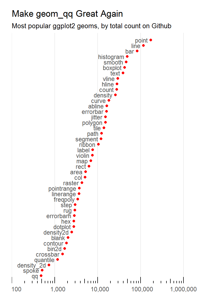
geoms <- geoms %>%
  mutate(
    result      = map(geom, w_msg(delay(search_gh))),
    total_count = map_int(result, "total_count")
)

## Processing: geom_text

## Processing: geom_vline

## Processing: geom_col

## Processing: geom_tile

## Processing: geom_qq

## ...

geoms

## # A tibble: 44 x 3
##           geom            result total_count
##          <chr>            <list>       <int>
##  1   geom_text <S3: gh_response>       38912
##  2  geom_vline <S3: gh_response>       29418
##  3    geom_col <S3: gh_response>        5088
##  4   geom_tile <S3: gh_response>       13993
##  5     geom_qq <S3: gh_response>         482
##  6  geom_label <S3: gh_response>        7703
##  7   geom_line <S3: gh_response>      116986
##  8 geom_smooth <S3: gh_response>       46169
##  9   geom_path <S3: gh_response>       12378
## 10  geom_spoke <S3: gh_response>         512
## # ... with 34 more rows

Finally, we plot the results.

ggplot(geoms, aes(x = total_count,
                  y = reorder(geom, total_count))) +
  geom_point(color = "red") +
  geom_text(
    aes(label = str_replace(geom, "geom_(.*)", "\\1  ")),
    size = 3,
    hjust = 1,
    color = "grey30"
  ) +
  scale_y_discrete(expand = c(0.03, 0)) +
  scale_x_log10(
    limits = c(100, 1500000),
    expand = c(0, 0),
    breaks = 10 ^ c(1:6),
    labels = format(10 ^ c(1:6),
                    scientific = FALSE, big.mark = ",")
  ) +
  annotation_logticks(sides = "b") +
  theme_minimal() +
  theme(
    axis.ticks.y = element_blank(),
    axis.text.y = element_blank(),
    panel.grid.major.y = element_blank(),
    panel.grid.minor.x = element_blank(),
    plot.margin = unit(rep(5, 4), "mm")
  ) +
  labs(
    x = NULL,
    y = NULL,
    title = "Make geom_qq Great Again",
    subtitle = paste0("Most popular ggplot2 geoms,",
                      " by total count on Github")
  )