Fixed points

In mathematics, a fixed point of a function is an element that gets mapped to itself by that function. For example, the function

\[ f : \mathbb{R} \rightarrow \mathbb{R} \] \[ f(x) = x^2 \]

maps the elements 0 and 1 to themselves, since \(f(0) = 0^2 = 0\) and \(f(1) = 1^2 = 1\).

To illustrate the concept, we could define a function fixed_points which maps functions to the set of their fixed points. We start, however, by defining a function approx_eq, which takes two vectors as input, does a pairwise check of equality within a given tolerance, and returns a boolean vector.

library(tidyverse)
library(gganimate)

approx_eq <- function(x, y, tol = 1e-2) {
  map2_lgl(x, y, ~isTRUE(all.equal(.x, .y, tolerance = tol)))
}

This roundabout solution is necessary in order to deal with the curious non-type-stable nature of all.equal which returns either TRUE or a character string explaining why the two elements are not equal!

With that in place, we now define fixed_points, which takes as input a function f and a domain x over which to evaluate f. It then returns all unique elements x that satisfy approx_eq(x, f(x)).

fixed_points <- function(f, x, ..., tol = 1e-2) {
    f_x <- f(x, ...)
    equal <- approx_eq(x, f_x, tol = tol)
    unique(x[equal])
}

f <- function(x) x^3

(fp <- fixed_points(f, -10:10))

## [1] -1  0  1

fp == f(fp)

## [1] TRUE TRUE TRUE

So we see that the function \(f(x) = x^3\) has the fixed points \({-1, 0, 1}\) over the interval \(-10 \leq x \leq 10\).

For convenience, and to see what’s really going on with the fixed points for various functions, we can define a function that plots a function and its fixed points (ggplot2 provides the convenient function stat_function for plotting arbitrary functions).

plot_fixed_points <- function(f, domain, ...) {
  fp <- fixed_points(f, domain, ...)
  
  ggplot(data.frame(x = domain), aes(x)) +
    geom_hline(yintercept = 0, size = 0.1) +
    geom_vline(xintercept = 0, size = 0.1) +
    stat_function(fun = f, color = "blue") +
    stat_function(fun = function(x) x, color = "red") +
    annotate("point", x = fp, y = fp) +
    annotate("text",  x = fp, y = fp, 
             label = sprintf("(%0.1f,%0.1f)", fp, fp),
             size = 3, hjust = -0.1, vjust = 2,
             check_overlap = TRUE) +
    coord_equal(ylim = range(domain)) +
    theme_minimal()
}

Let’s try it out on some common functions:

domain <- -10:10
plot_fixed_points(function(x) x^2, domain)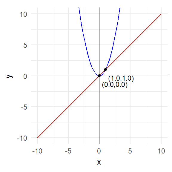

plot_fixed_points(function(x) x^3, domain)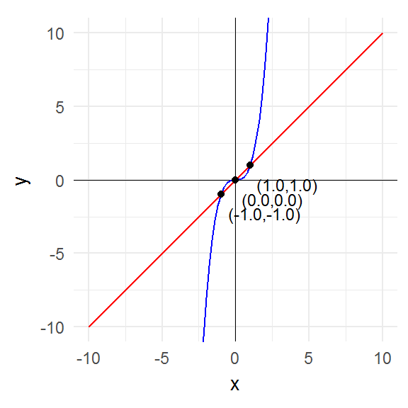

id <- function(x) x
plot_fixed_points(id, domain)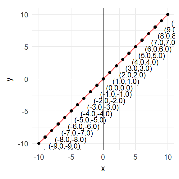

const_3 <- function(x) 3
plot_fixed_points(const_3, domain)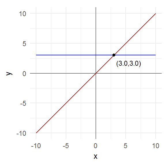

plot_fixed_points(abs, domain)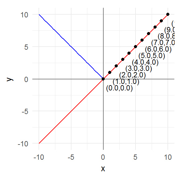

plot_fixed_points(sign, domain)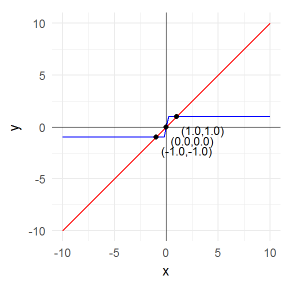

g <- function(x) x^4 + 3 * x^3 + x^2
domain2 <- seq(-4, 2, length.out = 1000)
plot_fixed_points(g, domain2)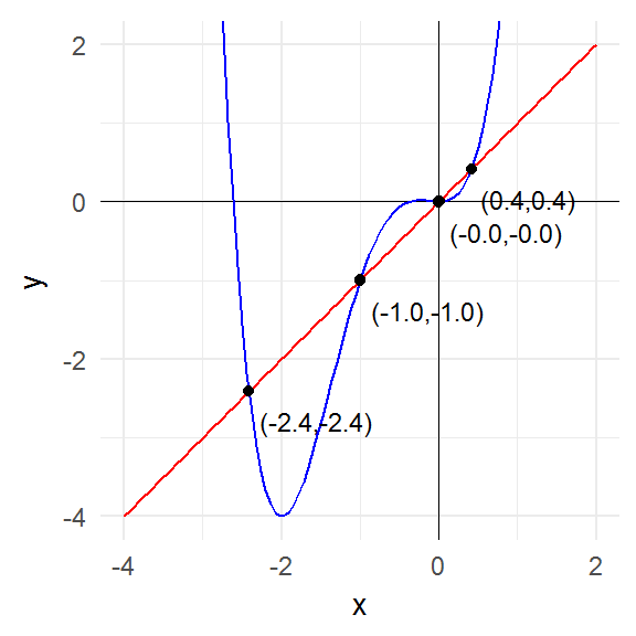

plot_fixed_points(sin, domain)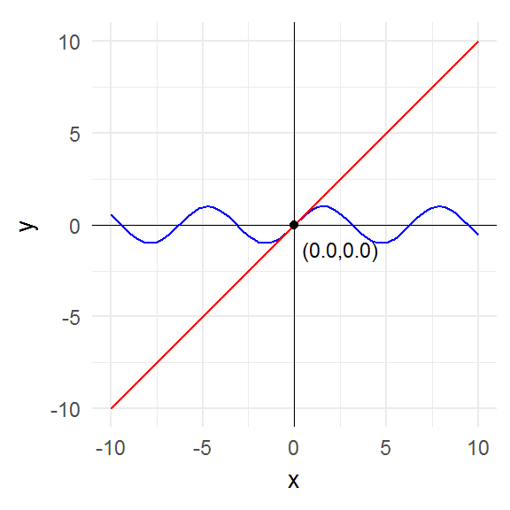

plot_fixed_points(cos, domain2)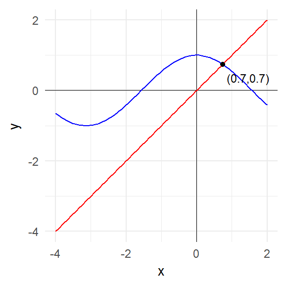

plot_fixed_points(function(x) x * (1 + sin(x)), 
                  seq(0, 20, 0.01))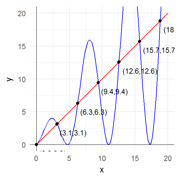

The key point to notice is that the fixed points are precisely those points where the graph of the function intersects the graph of the identity function (i.e. the 45° line).

Nothing stops us from applying fixed_points to non-numeric arguments. For example, we can confirm that the fixed points of toupper evaluated on all upper- and lower-case letters are exactly all the upper-case letters.

fixed_points(toupper, c(letters, LETTERS))

##  [1] "A" "B" "C" "D" "E" "F" "G" "H" "I" "J" "K" "L" "M" "N" "O" "P" "Q"
## [18] "R" "S" "T" "U" "V" "W" "X" "Y" "Z"