Using purrr to refactor imperative code - A blog about math and programming

Introduction

In a recent blog post, Nathan Eastwood solved the so-called Twitter Waterfall Problem using R. In his post, Nathan provides two solutions; one imperative approach using a large for-loop, and one more substantive approach using R6.

This post uses Nathan’s first solution as a case study of how to refactor imperative code using a more functional approach.

Problem

Consider this picture:

The blocks here represent walls, and we’re imagining what would happen if water were poured onto this structure. All water poured on the sides would run off, while some water would get trapped in the middle. In effect, it would end up looking like this:

So the problem is: given a set of walls, where would water accumulate?

Imperative solution

The walls are represented by a simple numerical vector wall. We then iterate over these walls from left to right. As Nathan explains,

The approach I took was one of many ways you could solve this problem. I chose to treat each column (wall) as an index and then for each index I implement a loop:

Find the height of the current index

Find the maximum height of the walls to the left of the current index

Find the maximum height of the walls to the right of the index

I then work out what the smallest maximum height is between the maximum heights to the left and right of the current index. If this smallest height minus the current index height is greater than zero, then I know how many blocks will fill with water for the current index. Of course, if the smallest maximum height to the left or right is less than the current height, then I get the run off.

Nathan offers the following solution (which I wrapped inside a function):

wall <- c(2, 5, 1, 2, 3, 4, 7, 7, 6)

get_water_original <- function(wall) {
  len <- length(wall)
  # pre-allocate memory to make the loop more efficient
  water <- rep(0, len)
  for (i in seq_along(wall)) {
    currentHeight <- wall[i]
    maxLeftHeight <- if (i > 1) {
      max(wall[1:(i - 1)])
    } else {
      0
    }
    maxRightHeight <- if (i == len) {
      0
    } else {
      max(wall[(i + 1):len])
    }
    smallestMaxHeight <- min(maxLeftHeight, maxRightHeight)
    water[i] <- if (smallestMaxHeight - currentHeight > 0) {
      smallestMaxHeight - currentHeight
    } else {
      0
    }
  }
  water
}

get_water_original(wall)

## [1] 0 0 4 3 2 1 0 0 0

The function outputs the correct solution, viz. that we would get water columns of height 4 in position 3, height 3 in position 4, and so on.

Functional solution

If we look closely at the for-loop we see that it really consists of three separate parts:

For a given i, find the current height, maximum height to the left, and maximum height to the right.
For a given set of heights, find the minimum of max heights to the left and the right, and find the difference between that and the current height.
Machinery for iterating over the wall vector and populating the water vector.

Having thus identified the relevant parts, we should be able to define/reuse three corresponding functions. We can use purrr::map to take care of all the looping machinery (point 3), so we just need to define functions get_heights and get_depth.

We first set a seed and load some packages.

set.seed(1)
library(tidyverse)
library(forcats)
library(microbenchmark)

Now, get_heights takes a vector wall and an index i as input, and starts by splitting up wall into left, right, and (implicit) mid parts. It then finds the maximum values for each part, and returns a list with the results.

get_heights <- function(wall, i) {
  left  <- wall[seq_len(i - 1)]
  right <- wall[seq(i + 1, length(wall))]
  list(l = max(left, 0, na.rm = TRUE),
       m = wall[i],
       r = max(right, 0, na.rm = TRUE))
}

get_heights(wall, 2)

## $l
## [1] 2
## 
## $m
## [1] 5
## 
## $r
## [1] 7

Next, get_depth takes a list of heights h produced by get_heights as input and returns either their least difference, or 0.

get_depth <- function(h) {
  max(min(h$l, h$r) - h$m, 0)
}

get_depth(get_heights(wall, 3))

## [1] 4

Since the co-domain of get_heights matches up with the domain of get_depth, we can now compose the two functions with purrr::compose to create a function f which takes as input a wall and an i and returns the depth of water at that position.

# equivalent to
# f <- function(wall, i) get_depth(get_heights(wall, i))
f <- compose(get_depth, get_heights)

Finally, we let map_dbl take care of the looping/iterating for us.

get_water <- function(wall) {
  map_dbl(seq_along(wall), f, wall = wall)
}

get_water(wall)

## [1] 0 0 4 3 2 1 0 0 0

In summary, then, we took a large for-loop and

split it up into two small, pure, encapsulated functions,
composed together those functions, and
mapped the composite function over the wall vector.

This, in my view, is the essence of functional programming.

Comparing results

We can test if the two solutions give identical results by generating a large wall and compare the results.

big_wall <- sample(1:1000, 1000, TRUE)
all(get_water_original(big_wall) == get_water(big_wall))

## [1] TRUE

We can also check whether one solution is faster than the other:

microbenchmark(get_water(big_wall), get_water_original(big_wall))

## Unit: milliseconds
##                          expr      min       lq     mean   median       uq
##           get_water(big_wall) 23.61028 25.01164 26.67536 25.36272 25.73384
##  get_water_original(big_wall) 10.32664 11.28836 11.99218 11.67553 11.84404
##       max neval
##  68.60116   100
##  53.56293   100

Unsurprisingly, the functional solution is somewhat slower, largely owing (presumably) to its greater number of function calls.

Plotting results

To plot a solution we first define a function that takes a wall as input, solves the problem, and returns a tidy data frame with all the necessary information for drawing the walls and water columns.

df_solution <- function(wall) {
  df <- data_frame(
    x = seq_along(wall),
    wall,
    water = get_water(wall)
  )
  gather(df, key, y, -x)
}

df_solution(wall)

## # A tibble: 18 x 3
##        x   key     y
##    <int> <chr> <dbl>
##  1     1  wall     2
##  2     2  wall     5
##  3     3  wall     1
##  4     4  wall     2
##  5     5  wall     3
##  6     6  wall     4
##  7     7  wall     7
##  8     8  wall     7
##  9     9  wall     6
## 10     1 water     0
## 11     2 water     0
## 12     3 water     4
## 13     4 water     3
## 14     5 water     2
## 15     6 water     1
## 16     7 water     0
## 17     8 water     0
## 18     9 water     0

We can then pass such a data frame into plot_solution to draw the walls and water.

plot_solution <- function(df) {
  ggplot(df, aes(x + 0.5, y, fill = fct_rev(key))) +
    geom_col(position = "stack", show.legend = FALSE, width = 1) +
    scale_fill_manual(values = c("steelblue", "grey")) +
    scale_x_continuous(breaks = seq_along(wall)) +
    scale_y_continuous(breaks = seq(0, max(wall), 1)) +
    theme_void() +
    theme(
      strip.text = element_blank(),
      panel.ontop = TRUE,
      panel.grid.major.x = element_line(colour = "white", size = 0.1),
      panel.grid.major.y = element_line(colour = "white", size = 0.1),
      plot.margin = unit(rep(0.1, 4), "cm")
    ) +
    coord_equal()
}

plot_solution(df_solution(wall))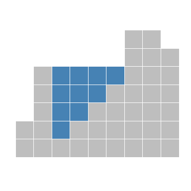

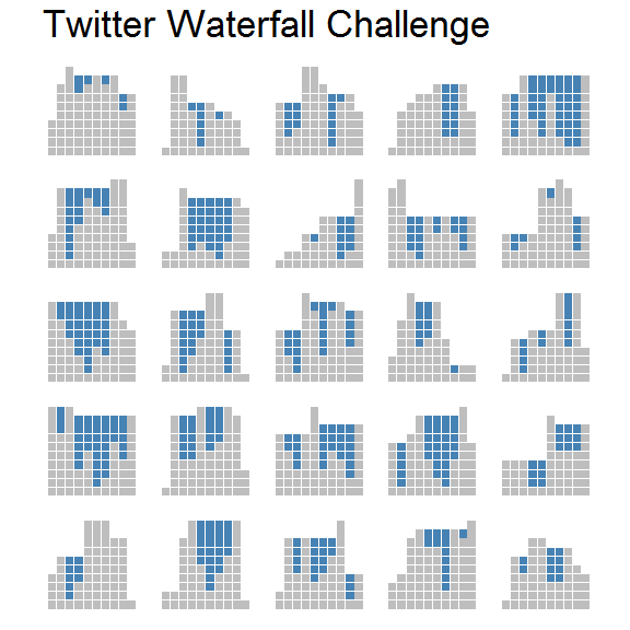
Finally, we can generate a large number of random walls and plot each solution as a separate facet.

walls <- rerun(25, df_solution(sample(1:10, 10, TRUE))) %>% 
  bind_rows(.id = "draw")

plot_solution(walls) +
  facet_wrap(~draw) +
  ggtitle("Twitter Waterfall Challenge")