XKCD and the normal distribution

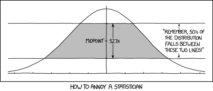
Thomas Lumley (@tslumley) has a nice blog post out today where he confirms the calculations of this XKCD picture:

In this post I do the same calculation, but take a somewhat different approach.

By exploiting the symmetry of the normal distribution, we can focus on calculating just the area in left part of the curve, and then double that to get the total area.

library(ggplot2)
theme_set(theme_classic())

g <- ggplot() + 
  stat_function(aes(-3:0), fun = dnorm) +
  geom_vline(xintercept = 0) +
  labs(x = NULL, y = NULL)

g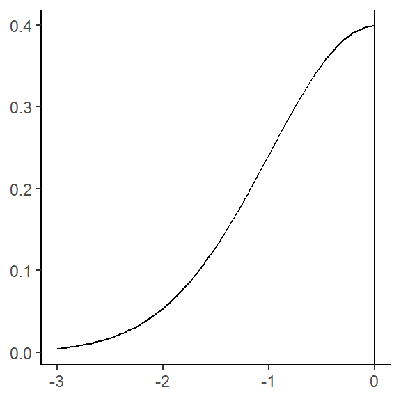

The XKCD picture tells us that the gray area is centered around the midpoint and constitute 52.7% of the total height of the curve evaluated at zero, i.e. \(\phi(0)\). That means that the heights of the remaining parts are \(\frac{1 - .527}{2}\) each.

h <- .527
k <- (1 - h) / 2
k

## [1] 0.2365

We can thus conclude that the horizontal lines have y-intercepts of:

q <- dnorm(0) * k
p <- dnorm(0) * (h + k)

g <- g +
  geom_hline(yintercept = c(p, q)) + 
  annotate("text", x = -3, y = c(p, q), 
           label = c("p", "q"), vjust = -1)

g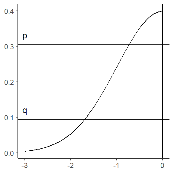

Next, we must find the x-values for where the horizontal lines intersect the density curve. This equivalent to finding the roots of the functions \(\phi(z) - q\) and \(\phi(z) - p)\):

a <- uniroot(function(z) dnorm(z) - q, c(-3, 0))$root
b <- uniroot(function(z) dnorm(z) - p, c(-3, 0))$root

g <- g + 
  geom_vline(xintercept = c(a, b)) +
  annotate("text", x = c(a, b), y = 0, 
           label = c("a", "b"), hjust = -1)

g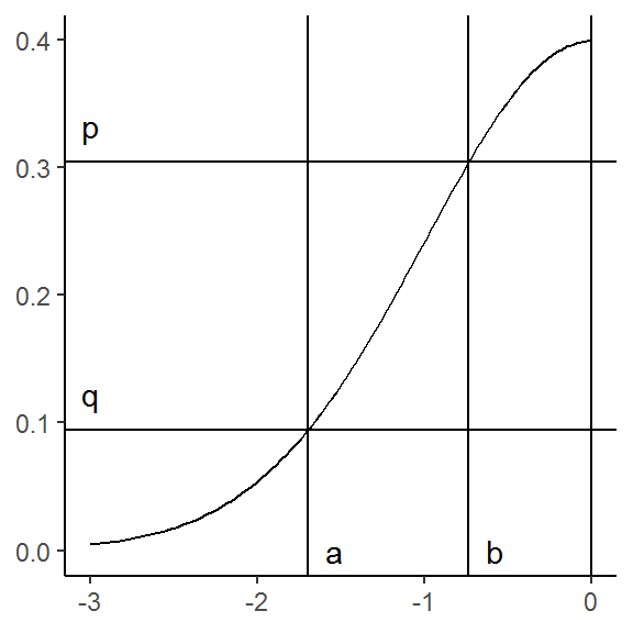

To keep things clear, we can now label the disjoint areas created by the intersecting lines:

g <- g +
  annotate("text", (a + b) / 2, q / 2,              label = "A") +
  annotate("text", b / 2      , q / 2,              label = "B") +
  annotate("text", b / 2      , (p + q) / 2,        label = "C") +
  annotate("text", b / 2      , (dnorm(0) + p) / 2, label = "D") +
  annotate("text", (a + b) / 2, (p + q) / 3,        label = "E")

g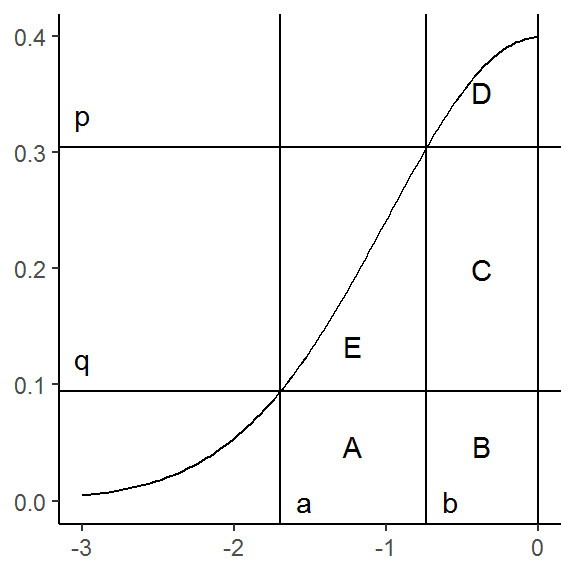

The areas of the rectangles are easy to calculate:

A <- abs(b - a) * q
B <- abs(b) * q
C <- abs(b) * (p - q)

To get the areas of E, however, we must integrate the normal curve between a and b, and then subtract the area of A:

\(\int_a^b \phi(z) dz - \int_a^b q dz.\)

This is equivalent to taking the difference between the normal CDF at a and b and subtracting A, i.e. \(\Phi(b) - \Phi(a) - A\). Similarly, we get the area of D by calculating \(\Phi(0) - \Phi(b) - (B + C)\)

E <- pnorm(b) - pnorm(a) - A
D <- pnorm(0) - pnorm(b) - (C + B)

With all areas calculated, we just need twice the area of \(C + E\):

total_area <- (C + E) * 2
sprintf("Total area: %0.2f%%", total_area * 100)

## [1] "Total area: 50.02%"

As expected, we get the correct result.