Introduction
I learned about this interesting problem from a recent blog post by @ryxcommar.
Imagine you have a time-series of the realized price of some stock:
library(ggplot2)

set.seed(2)
df <- data.frame(n = 1:100, y = cumsum(rnorm(100)))
head(df)
## n y
## 1 1 -0.8969145
## 2 2 -0.7120654
## 3 3 0.8757800
## 4 4 -0.2545957
## 5 5 -0.3348475
## 6 6 -0.2024272p <- ggplot(df, aes(x = n, y = y)) + geom_line()
p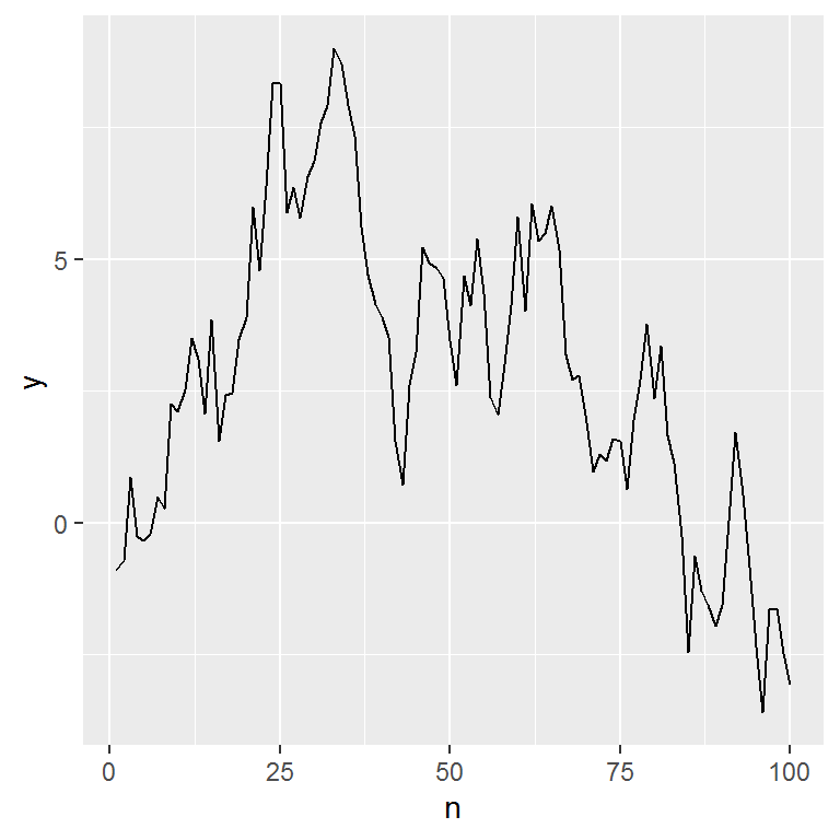
With the benefit of hindsight, when would’ve been the ideal period to buy and sell that stock? For this stock, inspection of the chart above suggests that the ideal trade would have been to have bought it in the first period, and sold it at the peak in period 33:
df_trade <- df[df$n %in% c(1, 33), ]
ggplot(df, aes(x = n, y = y)) +
geom_line() +
geom_line(data = df_trade, color = "red") +
geom_point(data = df_trade, color = "red")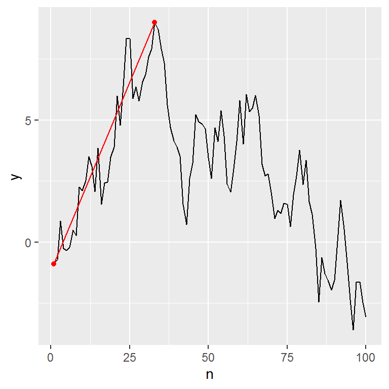
But how can we solve this problem in general? Also, how would the solution change if we were forced to hold the stock for \(N\) periods before being allowed to sell it?
In the original blog post, the author has two solutions; a naive solution based on a for-loop, and a preferred solution based on a series of table joins using SQL. In this post we will solve the same problem using some functional programming and a bit of matrix magic.
For kicks, we will solve it using base R for everything except plotting.
Solution strategy
Let’s first state the problem a bit more formally, mostly for notational purposes.
Problem
Let \(\overrightarrow{y} = [y_1, \dots, y_n]^T\) be a vector of length \(n\) with real-valued entries.
Find \(i, j \in \mathbb{N}^0\) such that \(i - j \geq N\), \(N \in \mathbb{N}\), and \(y_i - y_j \geq y_k - y_l\) for all \(k, l \in \{1, \dots, n\}\).
Solution
Let \(M\) be a matrix of pairwise differences of the elements in \(\overrightarrow{y}\):
\[ M = \begin{bmatrix} y_1 - y_1 & y_1 - y_2 & \dots & y_1 - y_n \\ y_2 - y_1 & y_2 - y_2 & \dots & y_2 - y_n \\ \vdots & \vdots & \ddots & \vdots \\ y_n - y_1 & y_n - y_2 & \dots & y_n - y_n \end{bmatrix} = \begin{bmatrix} 0 & -d_{21} & \dots & -d_{n1} \\ d_{21} & 0 & \dots & -d_{n2} \\ \vdots & \vdots & \ddots & \vdots \\ d_{n1} & d_{n2} & \dots & 0 \end{bmatrix}. \]
Now replace all entries of \(M\) above the diagonal with \(-\infty\):
\[ M' = \begin{bmatrix} 0 & -\infty & \dots & -\infty \\ d_{21} & 0 & \dots & -\infty \\ \vdots & \vdots & \ddots & \vdots \\ d_{n1} & d_{n2} & \dots & 0 \end{bmatrix}. \]
That is, choosing an “illegal” trade – where you sell the stock before you bought it – results in a payoff of negative infinity.
Let’s now assume that \(N = 0\), i.e. that that there are no restrictions on for how long we must hold the stock. With this assumption, and with \(M'\) constructed, all we need to do is extract the maximum value \(d_{ij}\) from \(M'\); \(i\) will be the sell-date, \(j\) the buy-date, and \(d_{ij}\) the realized profit.
As an aside for the algebra-heads among the readership, replacing illegal strategies with \(-\infty\) works because the extended real number line \(\bar{\mathbb{R}} = \mathbb{R} \cup \{-\infty, \infty\}\) forms a monoid under the maximum operator with \(-\infty\) as the identity element. The proof is left as an exercise.
Hint: you need to prove
- closure: \(\max(a, b) \in \mathbb{R} \cup \{-\infty, \infty\}\) for all \(a,b \in \bar{\mathbb{R}}\),
- associativity: \(\max(\max(a, b), c) = \max(a, \max(b,c))\) for all \(a,b,c \in \bar{\mathbb{R}}\),
- identity element: there exists some unique element \(e \in \bar{\mathbb{R}}\) such that \(\max(a, e) = \max(e, a) = a\) for all \(a \in \bar{\mathbb{R}}\).
Solution in R
With the solution strategy in hand, all we have to do now is implement it in R.
We first create a smaller data set to work with:
set.seed(3)
df <- data.frame(n = 1:10, y = cumsum(rnorm(10)))
df## n y
## 1 1 -0.9619334
## 2 2 -1.2544591
## 3 3 -0.9956709
## 4 4 -2.1478028
## 5 5 -1.9520200
## 6 6 -1.9218960
## 7 7 -1.8364783
## 8 8 -0.7198681
## 9 9 -1.9387255
## 10 10 -0.6713568p <- ggplot(df, aes(x = n, y = y)) + geom_line()
p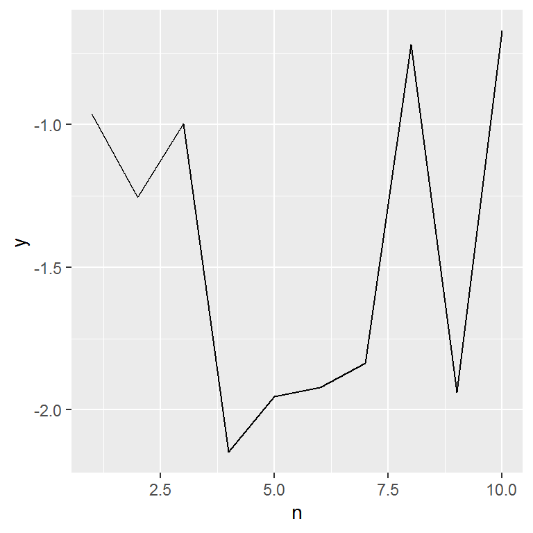
To create the matrix of pairwise differences we can use the generalized outer product (or “outer difference”) operator:
m <- outer(df$y, df$y, FUN = `-`)
round(m, 1)## [,1] [,2] [,3] [,4] [,5] [,6] [,7] [,8] [,9] [,10]
## [1,] 0.0 0.3 0.0 1.2 1.0 1.0 0.9 -0.2 1.0 -0.3
## [2,] -0.3 0.0 -0.3 0.9 0.7 0.7 0.6 -0.5 0.7 -0.6
## [3,] 0.0 0.3 0.0 1.2 1.0 0.9 0.8 -0.3 0.9 -0.3
## [4,] -1.2 -0.9 -1.2 0.0 -0.2 -0.2 -0.3 -1.4 -0.2 -1.5
## [5,] -1.0 -0.7 -1.0 0.2 0.0 0.0 -0.1 -1.2 0.0 -1.3
## [6,] -1.0 -0.7 -0.9 0.2 0.0 0.0 -0.1 -1.2 0.0 -1.3
## [7,] -0.9 -0.6 -0.8 0.3 0.1 0.1 0.0 -1.1 0.1 -1.2
## [8,] 0.2 0.5 0.3 1.4 1.2 1.2 1.1 0.0 1.2 0.0
## [9,] -1.0 -0.7 -0.9 0.2 0.0 0.0 -0.1 -1.2 0.0 -1.3
## [10,] 0.3 0.6 0.3 1.5 1.3 1.3 1.2 0.0 1.3 0.0Next, we need to replace the upper triangle with -Inf:
m[upper.tri(m)] <- -Inf
round(m, 1)## [,1] [,2] [,3] [,4] [,5] [,6] [,7] [,8] [,9] [,10]
## [1,] 0.0 -Inf -Inf -Inf -Inf -Inf -Inf -Inf -Inf -Inf
## [2,] -0.3 0.0 -Inf -Inf -Inf -Inf -Inf -Inf -Inf -Inf
## [3,] 0.0 0.3 0.0 -Inf -Inf -Inf -Inf -Inf -Inf -Inf
## [4,] -1.2 -0.9 -1.2 0.0 -Inf -Inf -Inf -Inf -Inf -Inf
## [5,] -1.0 -0.7 -1.0 0.2 0.0 -Inf -Inf -Inf -Inf -Inf
## [6,] -1.0 -0.7 -0.9 0.2 0.0 0.0 -Inf -Inf -Inf -Inf
## [7,] -0.9 -0.6 -0.8 0.3 0.1 0.1 0.0 -Inf -Inf -Inf
## [8,] 0.2 0.5 0.3 1.4 1.2 1.2 1.1 0.0 -Inf -Inf
## [9,] -1.0 -0.7 -0.9 0.2 0.0 0.0 -0.1 -1.2 0.0 -Inf
## [10,] 0.3 0.6 0.3 1.5 1.3 1.3 1.2 0.0 1.3 0So with these data, if we buy the stock in the first period and sell it in the
eight period, we’d realize a profit of 0.2 (m[8, 1]). The maximum appears in
m[10, 4], indicating that the optimum trade would have been to buy in period 4
and sell in period 10.
To extract the indices of the maximum we could first find the max in each column, and then find in what row that appears:
n_buy <- which.max(apply(m, 2, max))
n_sell <- which.max(m[, n_buy])
n_buy## [1] 4n_sell## [1] 10A nicer way, however, is to rely on the arr.ind argument of the which
function:
which(m == max(m), arr.ind = TRUE, useNames = FALSE)## [,1] [,2]
## [1,] 10 4Indeed, let’s wrap that into a function that follows our notation:
which.matrix.max <- function(m) {
idx <- which(m == max(m), arr.ind = TRUE, useNames = FALSE)
list(i = idx[, 1], j = idx[, 2])
}
trade <- which.matrix.max(m)
trade## $i
## [1] 10
##
## $j
## [1] 4Finally, we can add a line to the plot of the share price that connects the buying and selling periods:
df_trade <- df[df$n %in% c(trade$j, trade$i), ]
p +
geom_line(data = df_trade, color = "blue") +
geom_point(data = df_trade, color = "blue")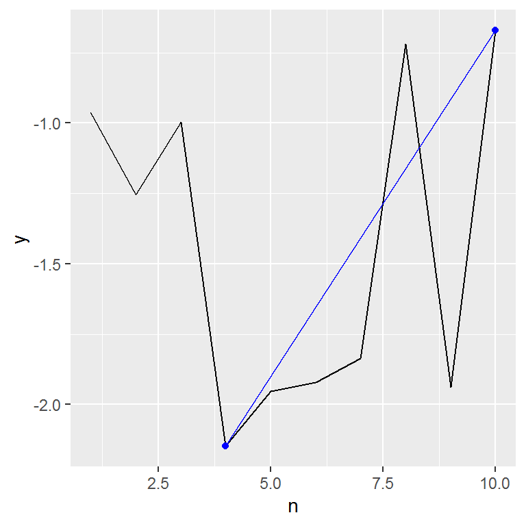
Generalizing the solution
What about if \(N > 0\)? That is, how does our strategy change if we are forced to
hold the stock for \(N\) periods before selling it (we’re also implicitly assuming
that we must make a trade at some point, i.e. we cannot choose to simply make no
trades)? Well, this simply amounts making the \(N\) entries below (and including
the diagonal) infeasible trades, so we simply have to set them to -Inf as
well.
If, for example, \(N = 7\):
N <- 7
m[row(m) - col(m) < N] <- -Inf
round(m, 1)## [,1] [,2] [,3] [,4] [,5] [,6] [,7] [,8] [,9] [,10]
## [1,] -Inf -Inf -Inf -Inf -Inf -Inf -Inf -Inf -Inf -Inf
## [2,] -Inf -Inf -Inf -Inf -Inf -Inf -Inf -Inf -Inf -Inf
## [3,] -Inf -Inf -Inf -Inf -Inf -Inf -Inf -Inf -Inf -Inf
## [4,] -Inf -Inf -Inf -Inf -Inf -Inf -Inf -Inf -Inf -Inf
## [5,] -Inf -Inf -Inf -Inf -Inf -Inf -Inf -Inf -Inf -Inf
## [6,] -Inf -Inf -Inf -Inf -Inf -Inf -Inf -Inf -Inf -Inf
## [7,] -Inf -Inf -Inf -Inf -Inf -Inf -Inf -Inf -Inf -Inf
## [8,] 0.2 -Inf -Inf -Inf -Inf -Inf -Inf -Inf -Inf -Inf
## [9,] -1.0 -0.7 -Inf -Inf -Inf -Inf -Inf -Inf -Inf -Inf
## [10,] 0.3 0.6 0.3 -Inf -Inf -Inf -Inf -Inf -Inf -InfNow the only feasible trades are to buy in one of the first three periods and sell in the last three periods. The best one would have been to buy in period 2 and sell in period 10.
Since the m[row(m) - col(m) < N] solution generalizes the use of upper.tri
above, we can wrap this into a function:
make_payoff_matrix <- function(x, N) {
m <- outer(x, x, FUN = `-`)
m[row(m) - col(m) < N] <- -Inf
m
}
m <- make_payoff_matrix(df$y, 7)
round(m, 1)## [,1] [,2] [,3] [,4] [,5] [,6] [,7] [,8] [,9] [,10]
## [1,] -Inf -Inf -Inf -Inf -Inf -Inf -Inf -Inf -Inf -Inf
## [2,] -Inf -Inf -Inf -Inf -Inf -Inf -Inf -Inf -Inf -Inf
## [3,] -Inf -Inf -Inf -Inf -Inf -Inf -Inf -Inf -Inf -Inf
## [4,] -Inf -Inf -Inf -Inf -Inf -Inf -Inf -Inf -Inf -Inf
## [5,] -Inf -Inf -Inf -Inf -Inf -Inf -Inf -Inf -Inf -Inf
## [6,] -Inf -Inf -Inf -Inf -Inf -Inf -Inf -Inf -Inf -Inf
## [7,] -Inf -Inf -Inf -Inf -Inf -Inf -Inf -Inf -Inf -Inf
## [8,] 0.2 -Inf -Inf -Inf -Inf -Inf -Inf -Inf -Inf -Inf
## [9,] -1.0 -0.7 -Inf -Inf -Inf -Inf -Inf -Inf -Inf -Inf
## [10,] 0.3 0.6 0.3 -Inf -Inf -Inf -Inf -Inf -Inf -InfWe can further combine this with the which.matrix.max above to encapsulate the
entire algorithm:
get_opt_trade <- function(x, N = 0) {
m <- make_payoff_matrix(x, N)
idx <- which.matrix.max(m)
data.frame(
n_buy = idx$j,
n_sell = idx$i,
n_held = idx$i - idx$j,
profit = x[idx$i] - x[idx$j],
N = N
)
}
get_opt_trade(df$y, 7)## n_buy n_sell n_held profit N
## 1 2 10 8 0.5831024 7Having abstracted away all the complexities of the solution, we can now easily ask, for example, how the optimum trade and profit changes as a function of the minimum holding period:
# Create a longer time-series
set.seed(11)
n <- 25
df <- data.frame(n = 1:n, y = cumsum(rnorm(n)))
p <- ggplot(df, aes(x = n, y = y)) + geom_line()
p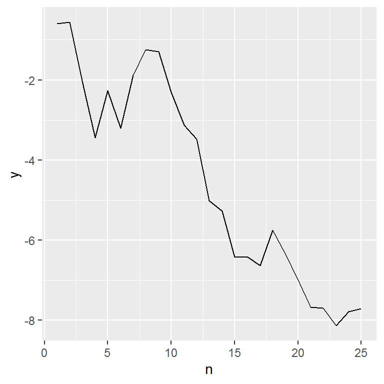
df_trade <- lapply(1:10, get_opt_trade, x = df$y)
df_trade <- do.call(rbind, df_trade)

df_trade <- merge(df_trade, df, by.x = "n_buy", by.y = "n")
df_trade <- merge(df_trade, df, by.x = "n_sell", by.y = "n",
                  suffixes = c("_buy", "_sell"))

p +
  geom_segment(aes(
    x = n_buy,
    xend = n_sell,
    y = y_buy,
    yend = y_sell,
    color = factor(N)
    ),
    df_trade) +
  theme(legend.position = "bottom") +
  labs(color = "Minimum \nholding period")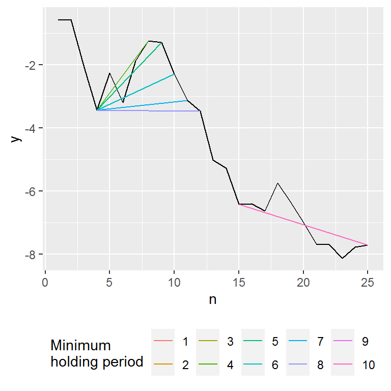
The chart shows an interest pattern. The simulated stock here slumped in the early period, peaked around periods 8-9, then fell almost monotonically afterwards. So if we faced no or only short minimum holding-limits, the best trade would have been to buy in the early slump and sell at the peak. However, if we’re forced to hold the stock for 9 or more periods, we would’ve been unable to conduct this trade. Our strategy then finds that the best trade (which minimizes losses) would have been to have bought and sold once the fall in stock prices had levelled off towards the end of the period.